Modeling Distributed Generation in the Buildings Sectors

Release date: December 2, 2020

Defining distributed generation

Distributed and dispersed generation technologies produce electricity near the load they are intended to serve, such as a residential home or commercial building. The U.S. Energy Information Administration (EIA) defines distributed generation (DG) as electricity generation that connects to the electric grid and is meant to directly offset retail sales. Dispersed generation is off-grid and is often used for remote applications where grid-connected electricity is cost-prohibitive. Dispersed generation in the buildings sector is not currently modeled in the National Energy Modeling System (NEMS), largely because of the difficulty in tracking installations and consumption.

One form of DG is combined heat and power (CHP), which reuses waste heat from onsite generation for purposes such as space heating and water heating. Such technologies are typically used in the commercial and industrial sectors.

Within the NEMS residential and commercial demand modules, DG is characterized as residential or non-residential. For modeling purposes in the Annual Energy Outlook 2020 (AEO2020), all non-residential, non-CHP installations are attributed to the commercial sector. DG modeled in NEMS includes both renewable and non-renewable technologies as outlined in Table 1.

Table 1: Distributed generation technologies by sector

	Residential	Commercial
Renewable	Solar photovoltaic Wind	Solar photovoltaic (PV) Wind Hydroelectric* Wood* Municipal solid waste*
Non-renewable	Natural gas-fired fuel cells	Natural gas-fired fuel cells Natural gas-fired reciprocating engines Natural gas-fired turbines Natural gas-fired microturbines Diesel reciprocating engines Coal*
Because of limited data availability and small amounts of penetration, hydroelectric, wood, municipal solid waste, and coal are aggregated into other DG technologies and are not explicitly characterized in this report.

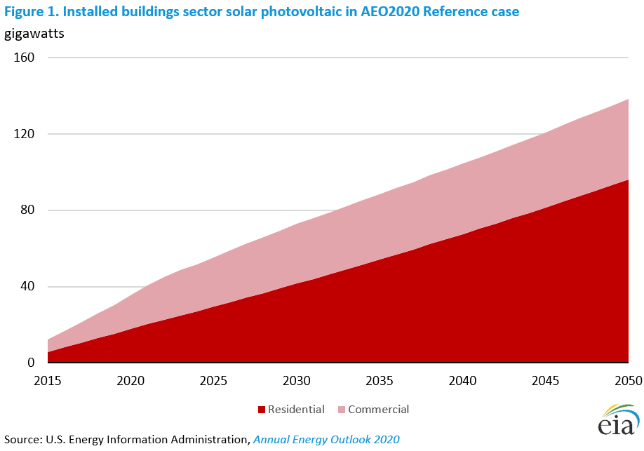
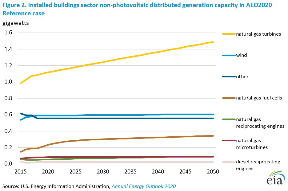
The residential and commercial demand modules of NEMS project capacity, generation, and fuel use of DG and CHP technologies. EIA develops these projections based in part on the economic returns projected for such equipment, as well as median household income, social spillover or imitation, and other effects for the residential sector. Figure 1 shows the projected capacity of solar photovoltaic (PV) in the AEO2020 Reference case, and Figure 2 shows the projected capacity of non-PV DG technologies.

The modules use a detailed cash-flow approach to estimate the internal rate of return for a DG investment and to evaluate either simple payback (commercial) or years to positive cash flow (residential natural gas fuel cells and wind). EIA estimates residential solar PV by using a ZIP code-level hurdle model in which the level of nearby installed capacity and number of households in a given area are also factors in PV penetration. Penetration assumptions for DG and CHP technologies are a function of the estimated rate of return relative to purchased electricity. In general, capital costs are characterized on a per-kilowatt basis minus available incentives.

The demand sectors of NEMS operate at the U.S. census division level but attempt to account for the wide variety of resource estimates, electricity and natural gas prices, and interconnection policies at local levels. Utility, state, and local incentives for DG are not explicitly characterized, but historical benchmarks ensure that the effects of past and existing incentive programs on an aggregate basis are included in the model.

Technology cost projections incorporate a concept known as technology learning (or learning-by-doing in economics), which assumes that cost declines may be expected as markets for DG technologies grow. For instance, EIA assumes in AEO2020 that fuel-cell and PV systems result in a 13% reduction in capital costs each time the installed capacity in the residential and commercial building sectors doubles (in the case of PV, utility-scale capacity is also included for learning). Doubling the installed capacity of microturbines results in a 10% reduction in capital costs, and doubling the installed capacity of distributed wind systems results in a 3% reduction. In this way, capacity increases can lead to projected cost reductions. However, the model also refers to a set of menu costs that represent a minimum assumed level of cost reduction and operates with this cost if it is lower than the cost produced by the technology learning function.

Historical capacity estimates

EIA also uses existing annual capacity estimates in the model to benchmark to recent history. EIA currently uses third-party sources to estimate historical capacity. For solar PV capacity, EIA depends on the published Solar Energy Industries Association (SEIA) state-level annual installed capacity estimates that are based on information from state agencies, utility programs, or incentive administrators. For wind, EIA uses the Distributed Wind Market Report, which provides national estimates of installed capacity published by the Pacific Northwest National Laboratory for the U.S. Department of Energy.

The historical reliance on third-party estimates of capacity reflects the gaps in historical coverage of installed capacity for distributed generators in data collected through EIA surveys of the electric power sector. Recently updated survey methodology may allow EIA to calculate a lower bound of the installed capacity. Form EIA-860 captures utility-scale installations in which plant capacity is greater than or equal to 1 megawatt, and Form EIA-861 captures net-metered installations of both distributed and dispersed generation in the residential sector and commercial/industrial sectors. This effort includes capacity attributed to third-party operators (TPOs) such as Tesla, Sunrun, and Vivint Solar. Again, for modeling purposes, EIA attributes all non-residential, non-CHP installations to the commercial sector. However, because of gaps in historical coverage by Form EIA-860 and Form EIA-861, EIA continues to use third-party data. The parameters for commercial distributed generation diffusion are calibrated to a historical data series beginning in 2004.

Costs and incentives

DG technology costs are generally characterized by an installed system cost for

• Main generating equipment (such as modules, turbines, or generators)
• Balance-of-system components
• Installation and permitting
• Replacement of major components such as inverters
• Ongoing annual maintenance

EIA primarily uses current and projected costs provided in contracted reports that are based on literature review, industry analysis, and discussions with manufacturers, distributors, and installers.¹ EIA uses additional reference sources (such as Lawrence Berkeley National Laboratory’s annual Tracking the Sun report² and the National Renewable Energy Laboratory’s Annual Technology Baseline³) to regularly update historical and projected cost assumptions for solar PV systems given the rapidly changing market for this technology.

The installed system cost is characterized on a per-kilowatt basis, and typical system capacities are assumed for each sector and technology type. The generating equipment and ancillary equipment, such as inverters, have separate expected lifetimes because ancillary equipment often does not last as long as the generating equipment.

Inputs are costs before subtracting any incentives. Because NEMS operates at the census division level, incentives available at the utility, state, and local levels are not directly included. EIA includes federal tax credits, however. Investment tax credits (ITCs) created by the Energy Policy Act of 2005 (EPACT05) and continued by the Energy Improvement and Extension Act of 2008 (EIEA08) and Consolidated Appropriations Act of 2016 (H.R. 2029) foster the growth of DG capacity. Solar PV, wind, and natural gas fuel cells receive a 30% tax credit under the ITC provisions of the EPACT05, which the H.R. 2029 legislation extended in December 2015. The five-year ITC extension for solar PV systems provided a 30% tax credit through 2019, which decreased to 26% in 2020 and will decreased to 22% in 2021. For commercial equipment only, the ITC will remain at 10% from 2022 onward. Residential equipment receives no ITC after 2021.

The residential and commercial modules use different criteria for determining levels of DG adoption. These different approaches reflect the differing methods used by individuals and businesses when making investment decisions. The residential module estimates penetration of solar PV units by using an econometric hurdle model, which uses ZIP code-level input data such as

• Median income
• Household population density
• Electricity rates
• Average annual solar irradiation
• Average mortgage interest rates
• Current installed PV capacity

For residential wind and natural gas fuel cell technologies, the residential module evaluates costs (after incentives) on number of years to net cumulative positive cash flow relative to purchasing electricity. The commercial module evaluates costs after incentives, based on internal rate of return (IRR) using a 30-year cash flow analysis to determine payback period for the different DG technologies. The model determines maximum market potential for each technology as a function of the payback period, then uses a Bass diffusion model (BDM) to project penetration as a fraction of overall maximum market potential. Studies have tested the BDM for fit against solar PV data and found a strong empirical relationship.⁴ The BDM uses two parameters—p, the coefficient of innovation, and q, the coefficient of imitation—to determine the shape of product penetration over time, according to the following equation:

$$

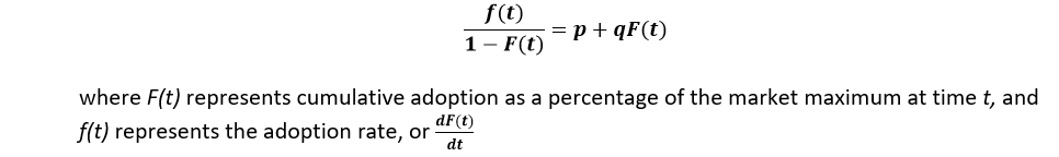
EIA estimated the p and q parameters in AEO2020 by census division and technology by using a non-linear least squares regression on historical capacity data.

EIA directly incorporates ITCs into the cash-flow approach for projecting distributed generation by residential natural gas fuel cells, wind, and all commercial DG technologies. The PV system cost net of any tax credits is used in the residential hurdle model when projecting the number of PV systems in the sector.

Interconnection potential

The DG submodules incorporate interconnection factors based on state-level policies intended to reflect the relative ease of contracting, constructing, and interconnecting DG. More than 45 states have some form of interconnection standard or guideline that governs how much DG capacity can be installed and incorporated into the electricity grid. The Database for State Incentives for Renewables and Efficiency (DSIRE) maintains a summary table for rules, regulations, and policies for renewable energy.⁵ EIA uses this table to generate a state’s score (out of 100) based on the presence of each of the policies listed below in Table 2.

Some states, such as California, had all of these policies and, therefore, received a score of 100. Alabama and Tennessee received the lowest scores; Alabama had none of the policies, and Tennessee had only one. These state-level scores are then population-weighted up to the census division level, translated into shares between 0 and 1, and applied to the penetration of DG in each division. These potentials improve over time based on historical rates of change in state-level interconnection policies.

Table 2. Distributed generation policies and interconnection potential weight

Policy	Weight
Net energy metering	30
Interconnection	25
Renewable portfolio standard (RPS)	25
Natural gas fuel cells or CHP in standards	10
Renewables access laws	10
Source: U.S. Energy Information Administration, Annual Energy Outlook 2020

Subregional niche markets

The NEMS residential and commercial demand modules model DG at the census division level; however, factors affecting the penetration of DG technologies can vary widely within a census division. For example, the Pacific Census Division, which includes Alaska, Hawaii, California, Oregon, and Washington, represents a wide variety of energy prices and climatic conditions. Average conditions for a census division may not appear to support economic penetration of these technologies, although actual economic penetration could be quite robust based on local conditions in niche areas.

Within the NEMS residential and commercial demand module, niche market factors attempt to account for local differences in characteristics affecting the penetration of DG, allowing for a more accurate representation when aggregating to census division levels. Some niche factors include:

• Average solar insolation
• Average wind speed
• Electricity rates relative to census division average
• Natural gas rates relative to census division average
• Average roof area per residential single-family household or unit of floorspace by commercial building type
• Share of rural households within each niche

EIA derived niche data from its 2012 Commercial Buildings Energy Consumption Survey (CBECS) and 2015 Residential Energy Consumption Survey (RECS) by overlaying each census division with solar insolation, wind speed, and climate zone maps. Because of greater CHP use in the sector, commercial resource niches are loosely based on subregions with similar climate conditions, as defined by heating degree days (HDDs) and cooling degree days (CDDs) provided in consumption survey microdata. EIA then mapped these subregions to their estimated solar insolation and wind speed. Because residential DG is dominated by solar PV capacity, residential niches are based first on average solar insolation.

Within each resource niche, EIA further mapped the microdata observations into subniches representing 10 commercial deciles and 3 residential electricity price levels. Each niche includes the share of floorspace within the census division for the commercial sector. Separate niche-level scaling factors for electricity prices and natural gas prices (commercial only) relative to the division average were applied to the projected census division price. Finally, for commercial PV, estimates of available roof area within each niche—based on a 2016 National Renewable Energy Laboratory report—were applied to total commercial floorspace.⁶ The module evaluates investment decisions and develops projected penetration for niches, and then it aggregates to obtain results for each census division. As mentioned in an earlier section, a separate ZIP code-level hurdle model is used to estimate residential PV installations; however, NEMS maintains the ability to use the residential cash flow model and subregional niches for comparison purposes.

Side cases

EIA refers to NEMS projections in which sets of assumptions are varied relative to the Reference case as side cases. Specific side cases show the effects of changing assumptions for DG. These cases use modified assumptions of

• Higher or lower economic growth
• Higher or lower oil and natural gas supply
• Higher or lower capital costs for renewable generation technologies

This section focuses on solar PV, which comprises the bulk of projected capacity additions and is more sensitive across cases than other DG technologies; however, EIA models all DG technologies across all side cases.

The High Economic Growth and Low Economic Growth cases for the AEO2020 reflect the effects of economic assumptions on energy consumption, which assume compound annual growth rates for U.S. gross domestic product of 2.4% and 1.4%, respectively, from 2019 to 2050, compared with 1.9% annual growth in the Reference case. In the High Oil and Gas Supply case, lower costs and higher resource availability than in the Reference case allow for higher production at lower prices. In the Low Oil and Gas Supply case, more pessimistic assumptions about resources and costs are applied. In the High Oil and Gas Supply case, the Henry Hub natural gas price in 2019 dollars is $2.54 per million British thermal units (MMBtu) in 2050, compared with $3.69/MMBtu in the Reference case and $6.56/MMBtu in the Low Oil and Gas Supply case.

AEO2020 includes a High Renewables Cost case and a Low Renewables Cost case, which examine sector sensitivities to capital costs for renewable generation technologies. The High Renewables Cost case assumes no capital cost reduction after 2019. The Low Renewables Cost case, on the other hand, assumes a more rapid cost reduction over time. In this case, capital costs fall by approximately 60% for residential and commercial solar PV between 2019 and 2050.

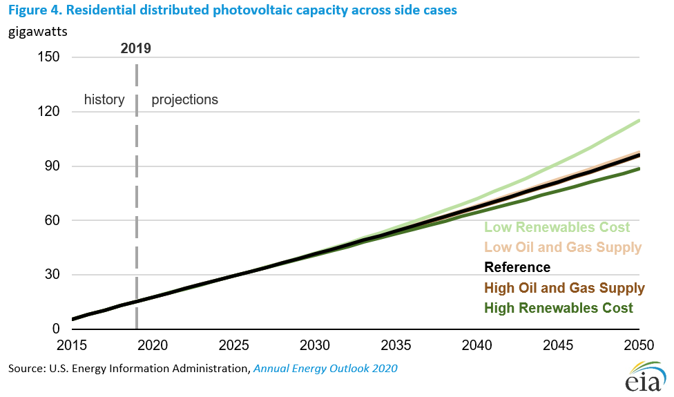
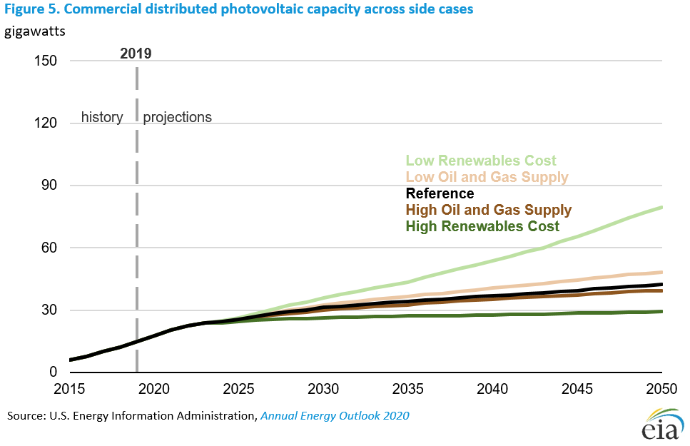
Figure 4 and Figure 5 compare the effects of individual side cases on PV projections. Capacity provides a good basis to compare PV adoption across technologies and alternative cases; however, a PV technology’s contribution to electricity generation may differ from its share of capacity additions. EIA projects the High Renewables Cost and Low Renewables Cost cases to have the greatest impact on both residential and commercial PV generation. Residential and commercial PV capacity in 2050 is projected to be 8% and 31% lower than the Reference case in the High Renewables Cost case and 20% and 87% higher in the Low Renewables Cost case, respectively. The Low Renewables Cost case also increases residential and commercial wind capacity in 2050, where projections are 186% and 40% higher than the Reference case, respectively. However, these increases are from a far smaller baseline than solar PV.

High or low natural gas prices, as reflected in the Low and High Oil and Gas Supply cases, affect the cost of electricity generation that DG displaces, and so they play a role in determining the value of these resources to the electric grid. The commercial delivered electricity price is higher in the Low Oil and Gas Supply case and lower in the High Oil and Gas Supply case compared with the Reference case. As a result, commercial solar capacity by 2050 is 14% more in the Low Oil and Gas Supply case and is 7% less in the High Oil and Gas Supply case compared with Reference case.

In the High Economic Growth case, residential and commercial solar capacity increase 1% and 4%, respectively, by 2050, compared with the Reference case. The additional capacity results from a combination of increased housing starts, real disposable personal income, and commercial floorspace.

An Issues in Focus article published as part of AEO2020 discusses the potential effects of alternative utility rate structures for compensating residential solar PV generation.

 

---

Footnotes

1. U.S. Energy Information Administration, Distributed Generation, Battery Storage, and Combined Heat and Power System Characteristics and Costs in the Buildings and Industrial Sectors, 2020.

2. Lawrence Berkeley National Laboratory, Tracking the Sun: Pricing and Design Trends for Distributed Photovoltaic Systems in the United States(October 2019).

3. National Renewable Energy Laboratory, 2019 Annual Technology Baseline(2019).

4. Wang, Wenyu, Nanpeng Yu, and Raymond Johnson, A Model for Commercial Adoption of Photovoltaic Systems in California, Journal of Renewable and Sustainable Energy 9:2 (2017).

5. North Carolina Clean Energy Technology Center, Database of State Incentives for Renewables & Efficiency(accessed June 22, 2020).

6. Gagnon, Pieter, Robert Margolis, Jennifer Melius, Caleb Phillips, and Ryan Elmore. 2016. “Rooftop Solar Photovoltaic Technical Potential in the United States: A Detailed Assessment.” National Renewable Energy Laboratory Technical Report (NREL/TP-6A20-65298).