Modeling Distributed Generation in the Buildings Sectors
Release date: November 7, 2017
Defining distributed generation
Distributed and dispersed generation technologies produce electricity near the particular load they are intended to serve, such as a residential home or commercial building. EIA identifies distributed generation (DG) as being connected to the electric grid and meant to directly offset retail sales. Dispersed generation is off-grid, often used for remote applications where grid-connected electricity is cost-prohibitive. Dispersed generation in the buildings sector is not currently modeled in the National Energy Modeling System (NEMS), largely because of the difficulty in tracking installations and consumption.
One form of DG is combined heat and power (CHP), which reuses waste heat from on-site generation for purposes such as space heating and water heating. Such technologies are typically used in the commercial and industrial sectors. The following information focuses on how EIA models DG, including CHP, in the residential and commercial sectors.
| Residential | Commercial | |
|---|---|---|
| Renewable | ||
| Non-renewable | ||
| * Due to limited data availability and isolated nature, hydroelectric, wood, municipal solid waste, and coal are aggregated into other DG technologies and are not explicitly characterized in this report. | ||
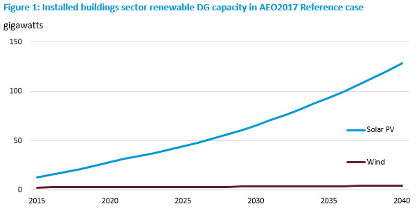
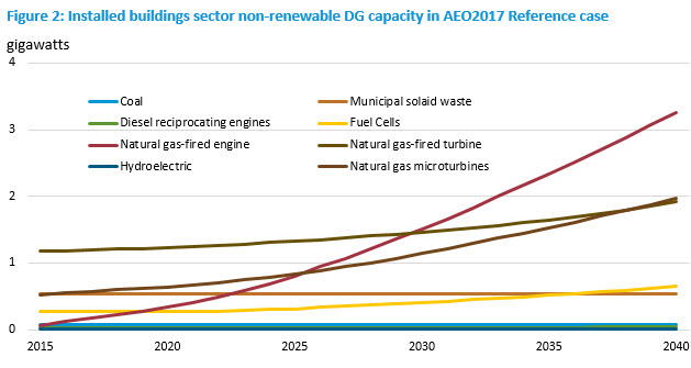
The residential and commercial demand modules of NEMS project capacity and generation of DG and CHP technologies. These projections are developed based on the economic returns projected for such equipment. Figure 1 shows the projected capacity of renewable DG technologies in the AEO2017 Reference case, and Figure 2 shows non-renewable PV DG technologies.
The modules use a detailed cash-flow approach to estimate the internal rate of return for an investment (commercial) or years to positive cash flow (residential fuel cells and wind). Residential solar PV is estimated using a ZIP code-level hurdle model in which the level of nearby installed capacity is also a factor in PV penetration. Penetration assumptions for DG and CHP technologies are a function of the estimated rate of return relative to purchased electricity. In general, capital costs are characterized on a per-kilowatt basis minus available incentives.
The demand sectors of NEMS operate at the U.S. Census division level but attempt to account for the wide variety of resource estimates, electricity and natural gas prices, and interconnection policies at more local levels. Utility, state, and local incentives for DG are not explicitly characterized, but historical benchmarks ensure that the effects of proven incentive programs on an aggregate basis are included in the model.
Technology cost projections incorporate a concept known as technology learning, which assumes that cost declines may be expected as markets for DG technologies grow. For instance, EIA assumes in AEO2017 that fuel-cell and PV systems result in a 13% reduction in capital costs each time the installed capacity in the residential and commercial building sectors doubles (in the case of PV, utility-scale capacity is also included for learning). Doubling the installed capacity of microturbines results in a 10% reduction in capital costs, and doubling the installed capacity of distributed wind systems results in a 3% reduction. In this way, capacity increases can lead to projected cost reductions. However, the model also refers to a set of menu costs that represent a minimum assumed level of cost reduction and operates with this cost if it is lower than the cost produced by the technology learning function (i.e., learned costs).Historical capacity estimates
Existing annual capacity estimates are also used in the model to benchmark to recent history. EIA currently uses third-party sources to estimate historical capacity. For solar PV capacity, EIA depends on the published Solar Energy Industries Association (SEIA) state-level annual installed capacity estimates that are based on information from state agencies, utility programs, or incentive administrators. For wind, EIA uses the Distributed Wind Market Report with national estimates of installed capacity published by the U.S. Department of Energy’s Pacific Northwest Laboratory.
The historical reliance on third-party estimates of capacity reflects the gaps in coverage of installed capacity for distributed generators in data collected through EIA surveys of the electric power sector. Recently updated survey methodology may allow EIA to calculate a lower bound of the installed capacity. Form EIA-860 captures utility-scale installations (i.e., where plant capacity is greater than or equal to 1 megawatt), and Form EIA-861 captures net-metered installations of both distributed and dispersed generation in the residential sector and commercial/industrial sectors. This effort now includes capacity attributed to third-party operators (TPOs) such as SolarCity, Sunrun, and Vivint Solar. Again, for modeling purposes, all non-residential, non-CHP installations are attributed to the commercial sector.Costs and incentives
DG technology costs are generally characterized by an installed system cost including the main generating equipment (e.g., modules, turbines, generators), balance-of-system components, and installation and permitting costs; replacement cost for major components such as inverters; and ongoing annual maintenance costs. EIA generally uses current and projected costs provided in contracted reports that are based on literature review, industry analysis, and discussions with manufacturers, distributors, and installers. Additional reference sources such as Lawrence Berkeley National Laboratory’s annual Tracking the Sun report and the National Renewable Energy Laboratory’s Annual Technology Baseline are used to annually update historical and projected cost assumptions for solar PV systems given the rapidly changing market for this technology.
The installed system cost is characterized on a per-kilowatt basis, with typical system sizes assumed for each sector and technology type. The generating equipment and ancillary equipment (i.e., inverters) have separate expected lifetimes, as inverters typically do not last as long as the generating equipment.
Inputs are provided as costs before any incentives. Because NEMS operates at the Census-division level, incentives available at the utility, state, and local levels are not directly included. Federal tax credits are assumed, however. Investment Tax Credits (ITCs) created by the Energy Policy Act of 2005 (EPACT05) and continued by the Energy Improvement and Extension Act of 2008 (EIEA08) and Consolidated Appropriations Act of 2016 (H.R. 2029) help to foster the growth of DG capacity. Solar PV, wind, and fuel cells receive a 30% tax credit, while engines, turbines, and microturbines receive a 10% ITC through 2016. The H.R.2029 legislation passed in December 2015 extends the ITC provisions of the Energy Policy Act of 2005 for renewable energy technologies. The five-year ITC extension for solar PV systems allows for a 30% tax credit through 2019, then decreasing to 26% in 2020, 22% in 2021, then remaining at 10% from 2022 onward for commercial equipment only. Residential equipment receives no ITC after 2021.
The residential and commercial modules use different criteria for determining levels of DG adoption. The residential module estimates penetration of solar PV units using an econometric hurdle model using ZIP code-level input data such as median income, household population density, electricity rates, average annual solar irradiation, average mortgage interest rates, and current installed PV capacity. For residential wind and fuel cell technologies, the residential module evaluates costs (after incentives) on number of years to net cumulative positive cash flow relative to purchasing electricity. The commercial module evaluates costs after incentives based on internal rate of return (IRR) using a 30-year cash flow analysis to determine payback period for the different DG technologies. Penetration assumptions are a function of this estimated IRR relative to purchased electricity. These different approaches are intended to reflect the differing methods used by individuals and businesses when making investment decisions.
ITCs are directly incorporated into the cash-flow approach for projecting distributed generation by residential fuel cells and wind and for all commercial DG technologies. The PV system cost net of any tax credits is used in the residential hurdle model in order to project the number of PV systems in the sector.Interconnection limitations
The DG submodules incorporate interconnection factors based on state-level policies that are intended to reflect the relative ease of contracting, constructing, and interconnecting DG. More than 45 states have some form of interconnection standard or guideline that governs how much DG capacity can be installed and incorporated into the electricity grid. The Database for State Incentives for Renewables and Efficiency (DSIRE) maintains a summary table for rules, regulations, and policies for renewable energy. This table is used to generate a state’s score (out of 100) based on the presence of each of the policies listed in Table 2 .
| Table 2: Distributed generation policies and interconnection limitation weight | |
|---|---|
| Policy | Weight |
| Net metering | 25 |
| Interconnection | 25 |
| Renewable Portfolio Standard | 25 |
| Fuel Cells or CHP in Standards | 10 |
| Access Laws | 10 |
| Public Benefits Fund | 5 |
Some states, such as California, had all of these policies and therefore received a score of 100. Two states, Alabama and Tennessee, only had one policy and received the lowest scores. These state-level scores are then population-weighted up to the Census-division level, translated into shares between 0 and 1, and used to limit the penetration of DG in each division. These limitations are lessened over time based on historical rates of change in state-level interconnection policies.
Commercial niche markets
The NEMS commercial demand module models DG at the Census division level; however, factors affecting the penetration of DG technologies can vary widely within a Census division. For example, the Pacific Census division, which includes Alaska and Hawaii in addition to California, Oregon, and Washington, represents a wide variety of energy prices and climatic conditions. Average conditions for a Census division may not appear to support economic penetration of these technologies, while actual economic penetration could be quite robust based on local conditions in niche areas.
Within the NEMS commercial demand module, niche market factors attempt to account for local differences in characteristics affecting the penetration of DG, allowing for a more accurate representation when aggregating to Census division levels. The niche factors include:
- solar insolation
- average wind speed
- electricity rates relative to Census division average
- natural gas rates relative to Census division average
- average roof area per unit of floorspace area by building type
Niche data were derived from the CBECS 2003 by overlaying climate zone maps for each Census division with solar insolation and wind speed maps. Rather than develop niches based on state-level borders, resource niches are loosely based on subregions with similar climate conditions, as defined by heating degree days (HDDs) and cooling degree days (CDDs) provided in the consumption survey observations. These subregions were then mapped to their estimated solar insolation and wind speed.
Within these resource niches, the microdata observations were further mapped into sub-niches representing below-average prices, average prices, and relatively high prices. Each niche includes the share of floorspace within the Census division for the commercial sector. Separate niche-level scaling factors for electricity prices and natural gas prices relative to the division average were applied to the projected Census division price. Finally, for PV, rough estimates of available roof area within each niche—based on building characteristics such as roof geometry and number of floors—were applied to total floorspace. The module evaluates investment decisions and develops projected penetration for niches, then aggregates to obtain results for each Census division.Side cases
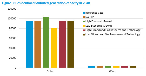
Several side cases show the effects of changing certain assumptions for DG, primarily projected fuel costs and macroeconomic scenarios. The AEO2017 also includes a No Clean Power Plan case to show how the absence of the U.S. Environmental Protection Agency’s policy could affect energy markets and emissions. Four side cases show the effects of changing assumptions not directly related to DG. These cases use Reference-level DG costs and policies, but they use modified assumptions of higher or lower economic growth and higher or lower oil or natural gas prices.
The High and Low Economic Growth cases reflect the effects of economic assumptions on energy consumption, which assume compound annual growth rates for U.S. gross domestic product of 2.6% and 1.6%, respectively, from 2016–40, compared with 2.2% annual growth in the Reference case. In the High Oil and Gas Resource and Technology case, lower costs and higher resource availability than in the Reference case allow for higher production at lower prices. In the Low Oil and Gas Resource and Technology case, more pessimistic assumptions about resources and costs are applied. In the High Oil and Gas Resource and Technology case, the Henry Hub Natural Gas price in 2016 dollars reaches $3.40 per million British Thermal Units (MMBTU) by 2040, compared to $5.07/MMBtu in the Reference case and $9.76/MMBtu in the Low Oil and Gas Resource and Technology case.
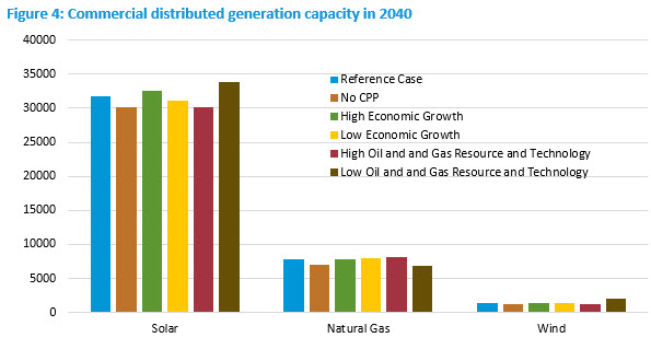
The effects of individual side cases can be compared in Figure 3 and Figure 4. Additional side cases are available in the Annual Energy Outlook side case tables. Capacity provides a good basis to compare DG adoption across technologies and alternative cases; however, a DG technology’s contribution to electricity generation may differ from its share of capacity additions. In the High Economic Growth case, by 2040 there is a 3% and 8% increase in solar capacity in the commercial and residential sectors, respectively, compared with the Reference case. These increases result from a combination of increased housing starts, real disposable personal income, and commercial floorspace.
High or low natural gas prices, as respectively reflected in the Low and High Oil and Gas Resource and Technology cases, affect the cost of electricity generation that DG displaces, and thus play a role in determining the value of these resources to the electric grid. Natural gas combined heat and power capacity in 2040 is 19% higher in the High Oil and Gas Resource and Technology compared to the Low case. This capacity increase results from the decrease in operating cost for the CHP technologies due to the decrease in natural gas prices. The commercial delivered electricity price is higher in the Low Oil and Gas Resource and Technology case compared to the Reference case, leading to higher levels of solar (7%) and wind capacity (49%) by 2040.