|
|
||||||||||||
|
The National Energy Modeling System: An Overview
|
Full Printer-Friendly Version |
|||||||||||
|
|
||||||||||||
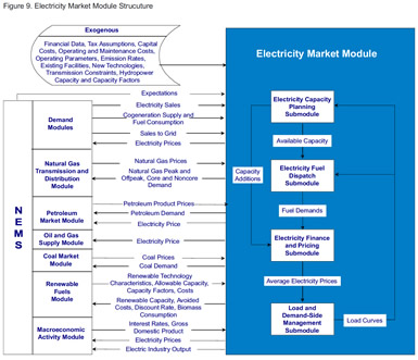
| Electricity Market Module | ||||||||||||
|---|---|---|---|---|---|---|---|---|---|---|---|---|
 |
|
|||||||||||
| Electricity Capacity Planning Submodule | back to top | |||||||||||
|
||||||||||||
| Electricity Fuel Dispatch Submodule | back to top | |||||||||||
|
||||||||||||
| Electricity Finance and Pricing Submodule | back to top | |||||||||||
The costs of building capacity, buying power, and generating electricity are tallied in the electricity finance and pricing (EFP) submodule, which simulates both competitive electricity pricing and the cost-of-service method often used by State regulators to determine the price of electricity. The AEO2009 reference case assumes a transition to full competitive pricing in New York, Mid-Atlantic Area Council, and Texas, and a 95 percent transition to competitive pricing in New England (Vermont being the only fully-regulated State in that region). California returned to almost fully regulated pricing in 2002, after beginning a transition to competition in 1998. In addition electricity prices in the East Central Area Reliability Council, the Mid-American Interconnected Network, the Southeastern Electric Reliability Council, the Southwest Power Pool, the Northwest Power Pool, and the Rocky Mountain Power Area/Arizona are a mix of both competitive and regulated prices. Since some States in each of these regions have not taken action to deregulate their pricing of electricity, prices in those States are assumed to continue to be based on traditional cost-of-service pricing. The price for mixed regions is a load-weighted average of the competitive price and the regulated price, with the weight based on the percent of electricity load in the region that has taken action to deregulate. In regions where none of the states in the region have introduced competition—Florida Reliability Coordinating Council and Mid-Continent Area Power Pool—electricity prices are assumed to remain regulated and the cost-of-service calculation is used to determine electricity prices. Using historical costs for existing plants (derived from various sources such as Federal Energy Regulatory Commission Form 1, Annual Report of Major Electric Utilities, Licensees and Others, and Form EIA-412, Annual Report of Public Electric Utilities), cost estimates for new plants, fuel prices from the NEMS fuel supply modules, unit operating levels, plant decommissioning costs, plant phase-in costs, and purchased power costs, the EFP submodule calculates total revenue requirements for each area of operation—generation, transmission, and distribution—for pricing of electricity in the fully regulated States. Revenue requirements shared over sales by customer class yield the price of electricity for each class. Electricity prices are returned to the demand modules. In addition, the submodule generates detailed financial statements. For those States for which it is applicable, the EFP also determines competitive prices for electricity generation. Unlike cost-of-service prices, which are based on average costs, competitive prices are based on marginal costs. Marginal costs are primarily the operating costs of the most expensive plant required to meet demand. The competitive price also includes a reliability price adjustment, which represents the value consumers place on reliability of service when demands are high and available capacity is limited. Prices for transmission and distribution are assumed to remain regulated, so the delivered electricity price under competition is the sum of the marginal price of generation and the average price of transmission and distribution. | ||||||||||||
| Electricity Load and Demand Submodule | back to top | |||||||||||
The electricity load and demand (ELD) submodule generates load curves representing the demand for electricity. The demand for electricity varies over the course of a day. Many different technologies and end uses, each requiring a different level of capacity for different lengths of time, are powered by electricity. For operational and planning analysis, an annual load duration curve, which represents the aggregated hourly demands, is constructed. Because demand varies by geographic area and time of year, the ELD submodule generates load curves for each region and season. |
||||||||||||
| Emissions | back to top | |||||||||||
EMM tracks emission levels for sulfur dioxide (SO2) and nitrogen oxides (NOx). Facility development, retrofitting, and dispatch are constrained to comply with the pollution constraints of the CAAA90 and other pollution constraints including the Clean Air Interstate Rule. An innovative feature of this legislation is a system of trading emissions allowances. The trading system allows a utility with a relatively low cost of compliance to sell its excess compliance (i.e., the degree to which its emissions per unit of power generated are below maximum allowable levels) to utilities with a relatively high cost of compliance. The trading of emissions allowances does not change the national aggregate emissions level set by CAAA90, but it does tend to minimize the overall cost of compliance. In addition to SO2, and NOx, the EMM also determines mercury and carbon dioxide emissions. It represents control options to reduce emissions of these four gases, either individually or in any combination. Fuel switching from coal to natural gas, renewables, or nuclear can reduce all of these emissions. Flue gas desulfurization equipment can decrease SO2 and mercury emissions. Selective catalytic reduction can reduce NOx and mercury emissions. Selective non-catalytic reduction and low-NOx burners can lower NOx emissions. Fabric filters and activated carbon injection can reduce mercury emissions. Lower emissions resulting from demand reductions are determined in the end-use demand modules. The AEO2009 includes a generalized structure to model current state-level regulations calling for the best available control technology to control mercury. The AEO2009 also includes the carbon caps for States that are part of the RGGI. |
||||||||||||
|
|
|||||||||||
|
||||||||||||