Overview

The square footage, or size, of a home is an important characteristic in understanding its energy use. The amounts of energy used for major end uses such as space heating and air conditioning are strongly related to the size of the home. The Residential Energy Consumption Survey (RECS), conducted by the U.S. Energy Information Administration (EIA), collects information about the size of the responding housing units as part of the data collection protocol. The methods used to collect data on housing unit size produce square footage estimates that are unique to RECS because they are designed to capture the energy-consuming space within a home. This document discusses how the 2015 RECS square footage estimates were produced.

Prior to the 2015 RECS, household interviews were conducted in person by trained interviewers. The interviewers measured the dimensions of the homes, then the measurements were used to calculate the square footage of the homes. However, the 2015 RECS household data were collected using a combination of three modes: traditional in-person computer-assisted personal interviews (CAPI), paper questionnaires sent through the mail, and web questionnaires. Because the surveys completed by paper and web were self-administered (completed by the respondent without the presence of an interviewer), it was not possible for an interviewer to measure the size of these homes as in previous survey cycles. As a result, square footage was imputed for about two-thirds of the 2015 RECS homes. The combination of the square footage measured by interviewers and the imputed data for self-administered surveys was used to produce estimates in the RECS data tables. These estimates are included for each household in the microdata file, with a flag that indicates whether a given household’s square footage was measured or imputed.

Specific topics covered in this document include:

• RECS square footage definitions
• The impact of using web and paper surveys for the 2015 RECS
• How interviewers measured housing units
• Technical details on the imputation for self-administered survey cases
• Data quality analysis
• Square footage data tables and variables in the public use file

EIA also considered alternatives to using the combination of measured and imputed data, including using estimates based on only data from CAPI household respondents, using third-party data, or modeling. These alternatives are discussed in Appendix A of this report.

The 2015 RECS household survey data collection, imputation, and square footage research were conducted in collaboration with IMG-Crown and RTI International.

Areas included in RECS square footage

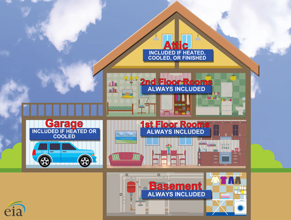
In RECS, total square footage, or floorspace, is a measurement of the two-dimensional area of the housing unit that is enclosed from weather by exterior walls, which is also where residential energy-consuming activities occur. Total square footage can be broken down into four areas: attic, basement, garage, and the rest of the home.

The basement and all living areas (the first floor, second floor, etc.) are always included in the RECS definition of square footage. Attics are only included if they are heated, cooled, or finished. Garages are only included if they are heated or cooled, and directly attached to the housing unit.

Figure 1: Areas included in RECS household square footage

Because of differences in definitions and methods, RECS square footage estimates may not be appropriate for comparison with other data sources. Most other surveys, including the American Housing Survey, rely on respondent estimates of a housing unit's size. Property tax records and real estate listings often rely on in-person measurements, but these included areas differ by jurisdiction and housing unit type and may focus on concepts like the useable space or livable space.

Methods used to collect and report 2015 RECS square footage data

All survey responses in iterations of RECS prior to 2015 were collected in person at the sampled household with a professionally-trained interviewer. The housing units were measured as part of the in-person household interview. The 2015 RECS is different from previous iterations of RECS in that a significant portion of the interviews were self-administered (completed on the web or by a paper survey). The use of self-administered modes significantly reduces the cost of RECS, as well as the time it takes to collect the data.

Of the 5,686 questionnaires completed in the 2015 RECS, 2,417 (42.5%) were completed in person with trained interviews, 2,122 (37.3%) were completed by web, and 1,147 (20.2%) were completed on paper. The addition of self-administered web and paper modes has implications in how square footage is collected because a trained interviewer did not measure the home.

The 2015 RECS square footage estimates were derived using a hybrid approach

The 2015 RECS square footage estimates in published data tables and the square footage values available in the public microdata file are derived using one of two methods. The method used was based on whether the interview was conducted in person or by a self-administered mode. Household square footage for the in-person interviews was collected using the same method as previous RECS, by the interviewer measuring the housing unit. The square footage for self-administered cases, almost 60% of all 2015 RECS cases, was imputed using the Predictive Mean Neighborhood (PMN) [1] hot-deck imputation method. Each method is described below.

Square footage was measured by interviewers when a household completed the in-person survey

For the 2015 RECS cases where the survey was completed in person, the interviewer measured the home. The respondent and interviewer first worked together to determine the number of stories in the housing unit, characteristics of the basement, attic, and garage, and the shape of each floor. Then the interviewer used a measuring tape to collect the dimensions of each floor of the housing unit.

Ideally, measurements were taken outside the housing unit to capture the total area of the home. Where outside measurements were not possible (for example, a high-rise apartment building), inside measurements were taken and adjusted for wall thickness after the interview. For standard-shaped floors (square, rectangle, T-, or L-shaped), the dimensions were recorded as part of the questionnaire on the interviewer's laptop. For floors with non-standard shapes, the interviewer sketched the shape on graph paper and recorded the necessary dimensions on the sketch.

Using the dimensions and sketches collected during the interview, a number of square footage components were calculated, including each floor's area, the attic, basement, and garage areas where applicable. The areas were summed to arrive at the total household square footage. The heated and cooled square footage was also derived based on other survey responses. Analysts reviewed unexpected or unusual values, as well as interviewer comments. When appropriate, dimensions were corrected to reflect accurately the size and shape of the housing unit.

Square footage was imputed when a household completed a self-administered survey

EIA used imputation to assign a value for in-person measured square footage to each home that completed the 2015 RECS by web or paper, even though self-reported square footage by respondents might be available. Imputation is the process of filling in the missing responses using a statistical model to produce a complete dataset and to reduce the bias associated with item nonresponse. The Predictive Mean Neighborhood (PMN) hot-deck imputation method was used to impute the missing 2015 RECS square footage values, as described in the section Technical details on imputation of square footage data below.

EIA studied other methods for reporting square footage for self-administered cases

EIA considered several other options for reporting square footage in the self-administered web and paper surveys and researched their feasibility. These options were:

• Using respondent estimates
• Using administrative data
• Using a model
• Using in-person measured data only

Technical details on imputation of square footage data

PMN hot-deck imputation conducted in a two-step process

Imputation, the process of filling in the missing responses using a statistical model, was used to assign measured square footage to the self-administered 2015 RECS households, as well as to surveys conducted in person where measurements were not available.[2] Imputation both produces a complete dataset and reduces the bias associated with item nonresponse.

The hot-deck imputation method was used for the 2015 RECS and previous survey cycles. In this method, a recipient case that has a missing value for the item being imputed is matched with a similar donor case that has a response. The donor's value for that item is used to replace the missing value for the recipient case.

There are various methods of applying hot-deck imputation that differ on how to group recipients and potential donors, and how to select the donor for a given recipient. For the 2015 RECS, a method called Predictive Mean Neighborhood (PMN) hot-deck imputation was used to derive the total square footage and its components for the self-administered cases, as well as for in-person surveys where measurements were not available. This two-step method combines prediction modeling and hot-deck imputation. Each step is described below.

Prediction modeling step

The first PMN step was to model the square footage values using linear regression based on a set of predictors and using the unit-nonresponse-adjusted weights (the sampling weights that have been adjusted to account for unit nonresponses). The goal in this step was to predict the mean (expected value of the square footage) for each case–both those that had measurements (the in-person survey respondents whose homes were measured by interviewers) and those that did not have measurements (web and paper survey respondents, as well as in-person survey respondents that did not have measurements). The predictors used in the regression model were characteristics of the housing unit related to square footage, such as the number of stories, number of bedrooms, number of windows, the year the house was built, and the respondent's estimate of their household square footage. The complete list of predictors for each housing unit type's model is included in Table 1: List of covariates used in PMN prediction modeling step.

Separate regression models were fitted for each housing type (single-family detached, single-family attached, apartment in a 2-4 unit building, apartment in a 5+ unit building, and mobile home) using cases from in-person surveys for which measured square footage was not missing. Predicted means were calculated for all records, both the cases that had measured square footage and the cases that did not. These values were then used in the next step (hot-deck imputation). Prediction modeling was implemented using specialized software called SUDAAN, which incorporated the unit nonresponse-adjusted weights and the complex survey design.

Table 1: List of covariates used in PMN prediction modeling step

Housing unit type	Covariates included in prediction model
Mobile homes	Square root of respondent's estimate of square footage, number of bedrooms, number of other rooms, number of weekdays someone is at home, number of windows, climate zone, year home was built, gender of householder, age of householder, race of householder, employment status of householder, household income, Census region, education level of householder, urban/rural indicator
Single-family detached	Square root of respondent's estimate of square footage, number of stories, number of household members, number of bedrooms, number of other rooms, number of weekdays someone is at home, presence of attic, presence of basement, presence of garage, number of windows, climate zone, year home was built, gender of householder, age of householder, race of householder, education level of householder, employment status of householder, household income, urban/rural indicator, Census region
Single-family attached	Square root of respondent's estimate of square footage, number of stories, number of household members, number of bedrooms, number of other rooms, number of weekdays someone is at home, presence of attic, presence of basement, presence of garage, number of windows, climate zone, year home was built, gender of householder, age of householder, race of householder, education level of householder, employment status of householder, household income, urban/rural indicator, Census region
Apartments in buildings with 2-4 units	Respondent's estimate of square footage, number of household members, number of bedrooms, number of other rooms, number of weekdays someone is at home, number of windows, climate zone, year home was built, gender of householder, age of householder, race of householder, education level of householder, employment status of householder, household income, urban/rural indicator, Census region
Apartments in Buildings with 5+ Units	Respondent's estimate of square footage, number of household members, number of bedrooms, number of other rooms, number of weekdays someone is at home, number of windows, climate zone, year home was built, gender of householder, age of householder, race of householder, education level of householder, employment status of householder, household income, urban/rural indicator, Census region

Hot-deck imputation step

The hot-deck imputation step of the PMN method selects a donor that has an expected value under the regression model close to that of a recipient record needing imputation that satisfies a set of logical and likeness constraints. These constraints prevent logical inconsistences between different variables in the data set, and they ensure the recipient and donor are as similar as possible.

First, the logical constraints were applied. An example of a logical constraint is that the donor and recipient must have the same number of stories in the house. After the logical constraints were applied, as many likeness constraints as possible were used to identify a small group of similar cases (the neighborhood). An example of a likeness constraint is that the donor and recipient have the same number of rooms in the home.

The selected donor was the case in the neighborhood with the closest predicted mean to the recipient (from the modeling step above). The donor's value of square footage then replaced the missing value of square footage in the recipient case.

Because square footage needed to be imputed for about two-thirds of the 2015 RECS cases (the self-administered cases plus the in-person cases where sufficient measurements were not taken), a larger pool of potential donors was desired. Therefore, the 8,600 cases from the 2009 RECS that had measured square footage were added to the dataset as part of the donor pool (see Data Quality section below).

Imputation rates

The overall imputation rate of the 2015 RECS household square footage variable is 65.6%. Imputation rates differ by housing unit type, ranging from 57.0% (in mobile homes) to 73.3% (in single-family attached homes), as shown in Table 2.

Table 2: 2015 RECS square footage measured and imputed rates

	Measured		Imputed
	Number	Percent	Number	Percent
Total	1,955	34.4	3,731	65.6
Mode of completion
In-person	1,955	80.9	462	19.1
Web/paper	0	0.0	3,269	100.0
Housing unit type
Mobile home	123	43.0	163	57.0
Single-family detached	1,231	32.8	2,521	67.2
Single-family attached	128	26.7	351	73.3
Apartment in 2-4 unit building	131	42.1	180	57.9
Apartment in 5+ unit building	342	39.9	516	60.1

PMN hot-deck an improvement over the 2009 RECS method

In the 2009 RECS, hot-deck imputation was also used for missing square footage in cases where the measurements were not available; however, the implementation was different from the PMN method. Instead of modeling square footage and grouping donors and recipients by the predicted mean values as in PMN, donors and recipients were grouped by having exact matches for multiple class variables. Class variables are variables that are related to the variable being imputed. For example, the number of floors in a home, whether it has a basement, the number of bedrooms in a home, and the region the home is in are related to square footage and were some of the class variables used. As a result, the values of these variables for the donors and recipients were exact matches.

The 2009 method also differed from PMN in how a final donor was selected from the pool of potential donors. PMN uses the statistical nearest neighbor method, while the 2009 method used Approximate Bayesian Bootstrapping.[3] In this method, a secondary donor pool is selected with replacement from the initial donor pool. The ultimate donor case is then randomly selected from this secondary donor pool.

The PMN method has several advantages over the 2009 method:

• It can accommodate more predictors and therefore has the potential to predict the mean of the missing item more accurately.
• The problem of sparse neighborhoods is reduced.
• Sampling weights can be easily incorporated in the models

Data quality analysis

EIA conducted an analysis to assess the data quality of the derived 2015 RECS square footage data using the hybrid approach of interviewer measured and imputed values.

The first part of the analysis was a simulation study done prior to the start of the 2015 RECS imputation that imputed a subset of the 2009 RECS cases that had measured square footage and compared the imputed and measured values. With the 2009 RECS cases that had measured square footage as the starting point, 100 simulation datasets were created, each with a subset of these square footage values set to missing using a logistic regression prediction model. The PMN hot-deck imputation method was used to impute these values, and the imputed and measured values were compared.

Table 3 shows the summary results of the simulation study. For all housing unit types except single-family attached, the difference of the imputed and reported means was less than 100 square feet, with an average relative bias of 5% or less in magnitude (see Appendix A for definition of relative bias). These differences are statistically significant for mobile homes, single-family detached, and apartments in 2-4 unit buildings; however, they are not large enough to be considered of practical importance.

The results of the study yielded a difference of means of 325 square feet and an average relative bias of 17% for single-family attached homes. The difference resulted from an unusually large single-family attached home measured by an interviewer in the 2009 dataset. This case was therefore used as a donor in the simulation study, even though it was uncommonly large for this type of home. This discovery led EIA to add a step to the 2015 RECS imputation process to remove unusually small or large outliers from the donor pool before the PMN imputation begins. These cases remained in the dataset as reported data but were not used as donors and therefore did not cause significant bias in the final data.

Table 3: Results of simulation study using PMN for 2009 RECS households

Housing unit type	Sample size**	Reported mean (square feet)	Imputed mean (square feet)	Difference of means (imputed minus reported)	Average relative bias
Mobile home	1,249	1,154	1,091	-62*	-5%
Single-family detached	67,901	2,766	2,856	90*	3%
Single-family attached	7,889	1,886	2,211	325*	17%
Apartment in building with 2-4  units	9,618	1,173	1,213	40*	3%
Apartment in building with 5+ units	17,642	820	825	5*	1%
* Indicates a statistically significant difference at the 5% level of significance ** From 100 simulated datasets

The second part of the analysis compared average square footage estimates from 2009 to the averages from 2015, overall and by geographic areas, climate regions, and housing type. Large, systematic differences could potentially indicate that the change in data collection protocol from 2009 to 2015 is problematic. However, as newer homes are generally larger than older homes, average home size would be expected to increase over time.

The average square footage estimate for all homes increased by 41 square feet (2.1%) from 2009 to 2015, not a statistically significant change. Most comparisons of 2009 square footage averages with 2015 square footage averages by geographic area were not statistically significant, with the exception of the West South Central Census division, which increased 155 square feet; the West Census region, which increased 78 square feet; and the Pacific Census division, which increased 80 square feet. By climate region, there were no statistically significant changes in housing size.

When comparing 2009 averages to 2015 averages by housing unit type, single-family detached homes, apartments in 2-4 unit buildings, and mobile homes had statistically significant changes, although the differences were all less than 100 square feet.

In summary, there do not appear to be square footage data quality issues in the 2015 RECS. A simulation study using the 2009 data shows that the PMN imputation method produced imputed average square footage estimates less than 100 square feet different from the measured average square footage values for all housing unit types, except single-family attached homes. The bias observed for single-family attached houses was due to some very large and very small square footage outlier values. For the 2015 imputation, removing outliers fixed the bias issue with single-family attached homes. Comparisons of average square footage estimates from the 2009 RECS with averages from the 2015 RECS do not produce any large or systematic differences that might indicate the change in the data collection protocol or in the imputation method is problematic. Although there are differences for some subpopulations, like mobile homes or the marine climate region, these differences were not large enough to prevent implementing these methods. Also, this method produced more reliable results than the alternative methods. These alternative methods are discussed in Appendix A.

Table 4: Comparison of final 2009 RECS and 2015 average square footage estimates*

	2009 RECS average	2015 RECS average	Difference (2015 - 2009)	% difference (2015 - 2009) / 2009
All homes	1,971	2,012	41	2.1%
Census region and division
Northeast	2,121	2,109	-12	-0.6%
New England	2,232	2,188	-44	-2.0%
Middle Atlantic	2,080	2,080	0	0.0%
Midwest	2,272	2,279	7	0.3%
East North Central	2,251	2,253	2	0.1%
West North Central	2,317	2,337	20	0.9%
South	1,867	1,941	74	4.0%
South Atlantic	1,944	2,007	63	3.2%
East South Central	1,895	1,860	-35	-1.8%
West South Central**	1,717	1,872	155	9.0%
West**	1,708	1,786	78	4.6%
Mountain	1,928	1,998	70	3.6%
Mountain North	2,107	2,130	23	1.1%
Mountain South	1,751	1,866	115	6.6%
Pacific**	1,605	1,685	80	5.0%
Climate region
Very cold/Cold	2198	2,239	41	1.9%
Mixed-humid	2,061	2,063	2	0.1%
Mixed-dry/Hot-dry	1,631	1,665	34	2.1%
Hot-humid	1,690	1,754	64	3.8%
Marine	1,676	1,853	177	10.6%
Housing unit type
Single-family detached	2,483	2,559	76	3.1%
Single-family attached	1,769	1,778	9	0.5%
Apartments  in buildings with 2-4 units**	1,100	1,024	76	-6.9%
Apartments  in buildings with 5 or more units	849	880	31	3.7%
Mobile homes**	1,087	1,183	96	8.8%
* Final RECS square footage estimates, which are shown in this table and in official RECS published tables and reports, excludes unconditioned space in garages. Simulations and actual imputation were done based upon the definition of individual measured levels of each home that included all garages. ** Indicates a statistically significant difference at the .05 level of significance Source: U.S. Energy Information Administration, 2009 and 2015 Residential Energy Consumption Surveys, Table HC10.9, values have been rounded to the nearest whole number.

Square footage data tables and variables in the public use file

Total and average 2015 RECS household square footage estimates are available in the online summary tables. The square footage variables are also included on the public use microdata file for custom user analysis. The variables included on the file are shown in Table 5. The variable TOTSQFT_EN is the total square footage including the main living space, all basements, garages if they are heated or cooled, and attics if they are heated, cooled, or finished. TOTSQFT_EN is the variable that was imputed with the PMN process; the other variables were derived from TOTSQFT_EN and other household variables.

Table 5: 2015 RECS square footage variables on the public use microdata file

Variable name	Variable description	Response codes and labels
TOTSQFT	Total square footage (includes all attached garages, all basements, and finished/heated/cooled attics)	Square feet
TOTSQFT_EN	Total square footage (includes heated/cooled garages, all basements, and finished/heated/cooled attics). Used for EIA data tables.	Square feet
TOTHSQFT	Total heated square footage	Square feet
TOTUSQFT	Total unheated square footage	Square feet
TOTCSQFT	Total cooled square footage	Square feet
TOTUCSQFT	Total uncooled square footage	Square feet
ZTOTSQFT	Imputation flag for TOTSQFT	0 Not Imputed 1 Imputed
ZTOTSQFT_EN	Imputation flag for TOTSQFT_EN	0 Not Imputed 1 Imputed
ZTOTHSQFT	Imputation flag for TOTHSQFT	0 Not Imputed 1 Imputed
ZTOTUSQFT	Imputation flag for TOTUSQFT	0 Not Imputed 1 Imputed
ZTOTCSQFT	Imputation flag for TOTCSQFT	0 Not Imputed 1 Imputed
ZTOTUCSQFT	Imputation flag for TOTUCSQFT	0 Not Imputed 1 Imputed

Each square footage variable has a corresponding imputation flag called a Z variable, which informs the data user whether a value was imputed or not imputed for a case. If the Z variable is 0, the value was not imputed; if it is 1, the value was imputed. For example, the Z variable for TOTSQFT_EN is ZTOTSQFT_EN. If ZTOTSQFT_EN for case xyz is 0, the value for TOTSQFT_EN was measured by the interviewer for case xyz and not imputed. If ZTOTSQFT_EN for case xyz is 1, the value for TOTSQFT_EN for case xyz was imputed.

Appendix A: Research on alternative methods for reporting square footage estimates

Alternative methods researched

EIA considered several other options for reporting square footage as an alternative to the hybrid approach described in this report:

• Using respondent estimates
• Using administrative data
• Using a model
• Using in-person measured data only

Each option is summarized below.

Respondent estimates

The RECS includes a question asking for the square footage of the respondent's home: "About how many square feet is your home? Your best estimate is fine." The respondent's estimate could potentially be used in place of interviewer-measured square footage.

Third-party data

Three data sources that have household square footage were evaluated for use in RECS: Zillow.com, Acxiom, and CoreLogic[4]. The square footage values from these administrative sources were options considered for the self-administered cases that did not have interviewer-measured data.

Model based

EIA considered model-predicted square footage as another potential replacement for interviewer-measured square footage. Two types of models were constructed—linear models and regression trees. The predictors for these models included questionnaire and frame data that were available for all cases. The dependent variable for the linear models was the RECS definition of household square footage. The dependent variables for the regression trees were the absolute and relative bias measures between the measured square footage estimate and the respondent estimate.

In-person measured data only

Another option for handling the problem of missing square footage data for self-administered cases was to only use the in-person measurements of square footage with the separate in-person sampling weights. Because the in-person sampling weights represent the entire population, the in-person square footage measurements can be used to estimate statistics like average square footage, median square footage, energy consumption per square foot, and total square footage of the U.S. household population.

Results of research project

EIA compared the respondent estimates, administrative data, and modeled data to the measured square footage for all in-person surveys completed in the 2009 and 2015 RECS. The measured square footage is considered  the gold standard. The bias and reliability were calculated to compare the quality of the data from these alternative options to the gold standard.

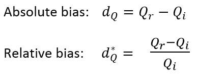
Bias and reliability definitions

Both absolute bias and relative bias were measured. Absolute bias is the difference between the alternative square footage (from the respondent estimate, administrative source, or modeled result) and the interviewer measurement; relative bias is the proportional difference between the alternative square footage and the interviewer measurement. These may be written as:

             where

             Q is the square footage for each respondent as measured by the interviewer (i) or the alternative measure (r)

              d is the difference between the estimates (Q) as calculated systematically or as a percentage of the interviewer
              measurement (*).

Absolute bias provides an overall magnitude of the difference between the alternative source of square footage (respondent estimate, administrative source, or modeled result) and interviewer measurement. It is also useful within subcategories of housing units where size is relatively similar (e.g., mobile homes). However, relative bias controls for differences in unit size. A respondent may misreport by 100 square feet. The importance of that difference is much greater if the respondent lives in a 500 square foot apartment than if he or she lives in a 5,000 square foot house; this difference can be observed using relative bias.

In addition to bias, the reliability of the alternative option square footage was also assessed. It is possible for both the interviewer measurement and the alternative square footage measure to be similar on average, producing an unbiased estimate, but have large differences for any given case. Consider the simple example of two cases that have interviewer-measured values of 900 and 1,000 square feet and respondent estimates of 600 and 1,300 square feet. Although both variables have a mean of 950 square feet, the respondent estimates are not reliable. Using the alternative measure in analyses may bias findings or alter the observed relationships. Reliability of the alternative measure can be written as:

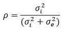
where

   We define e as the error in using Q_r to measure Q_i, which can be expressed mathematically as Q_r = Q_i + e.

    The denominator of  p is the variance of Q_r, which is the sum of the variance of the interviewer measurement() and the
   variance of the difference between the interviewer and alternative measures(), assuming that  and e are uncorrelated.

Analysis of respondent estimates

Analysis of the respondent estimates shows substantial bias and reliability issues. Table 6 shows the bias and reliability measures from the 2009 and 2015 RECS overall and by the subgroups of housing unit type and size. In 2009, respondents reported an average unit size of 1,671 square feet, compared to an average size of 2,098 square feet as measured by the interviewer. This difference produced an average underestimate of 427 square feet, consistent with the 2015 findings and the findings across all subgroups. In 2015, respondent reports were an average of 371 square feet less than measured square footage. In 31 of the 32 comparisons made across years and subgroups, the average respondent estimate is lower than the measured square footage estimate (the exception: 2015, mobile homes). Twenty-seven of these differences were significant at the 5% significance level.

Table 6: Bias and reliability of respondent estimates of square footage in the 2009 and 2015 RECS

		Respondent estimate (SQFTEST)	Measured square footage (TOTSQFT_EN)
	Number of homes	Mean	Mean	Reliability	Absolute Bias	Average relative Bias
2009
Overall	9,773	1,671	2,098	69.0%	-427	-11.0%
Housing unit type
Mobile homes	398	1,079	1,083	64.4%	-4	2.3%
Single family homes - detached	6,679	1,965	2,521	65.2%	-556	-14.1%
Single family homes - attached	700	1,384	1,790	59.3%	-407	-14.7%
Apartments in 2-4 unit buildings	591	937	1,117	57.0%	-180	-7.0%
Apartments in 5+ unit buildings	1,405	854	891	62.1%	-37	0.1%
Housing unit size (SQFTEST)
1 - 1,000 square feet	2,588	778	1,016	80.2%	-238	-13.2%
1,001 - 1,500 square feet	2,657	1,285	1,697	51.4%	-412	-13.2%
1,501 - 2,100 square feet	2,220	1,827	2,304	51.6%	-476	-10.5%
2,101 square feet or larger	2,308	2,967	3,573	58.0%	-60	-6.4%
2015
Overall	1,775	1,715	2.085	58.8%	-371	-8.2%
Housing unit type
Mobile homes	77	1,101	1,052	50.3	49	7.8%
Single family homes - detached	1,248	2,007	2,504	52.2%	-497	11.3%
Single family homes - attached	123	1,389	1,701	66.7%	-312	-12.1%
Apartments in 2-4 unit buildings	77	1,010	1,029	38.2%	-19	3.6%
Apartments in 5+ unit buildings	250	865	892	53.2%	-28	-0.1%
Housing unit size (SQFTEST)
1 - 1,000 square feet	450	750	1,032	72.6%	-283	-16.1%
1,001 - 1,500 square feet	500	1,276	1,710	51.3%	-434	-12.6%
1,501 - 2,100 square feet	398	1,818	2,407	50.9%	-589	-11.8%
2,101 square feet or larger	427	3,168	3,351	40.6%	-183	8.8%

The bias and reliability depend on housing unit type and housing unit size. Estimates from respondents living in single-family homes (both attached and detached) were the most biased, underestimating home size by an average of 312 to 556 square feet (depending on year and whether it was attached or detached). Apartment dwellers fared better. The average 2015 respondent estimates among apartments lacked evidence of bias, but the reliability of the respondent reports was still low (38.2% and 53.2% for apartments in small and large buildings, respectively).

Looking at mobile homes, it appears there is no bias among mobile homes in 2009 or 2015. On the surface, this lack of bias suggested that individuals living in mobile homes know the unit's size. Digging a little deeper, the range of the absolute bias among 2009 mobile home dwellers was 3,702 square feet (bias ranged from an underestimate of 1,840 square feet to an overestimate of 1,862 square feet), or 295%. The reliability of the respondent estimate compared to the measured square footage estimate was only 64.4%. In other words, 35.6% (1-0.644) of the variance of the respondent estimate is the result of measurement error and does not represent the variance of the gold standard.

This finding was not unique to mobile home dwellers. In the overall estimates, the reliability was 69.0% and 58.8% for 2009 and 2015, respectively. Although a linear trend between respondent and the measured square footage estimate exists, it is far from exact.

Although the average respondent report was biased among 2009 apartments in buildings with five or more units, the difference was small (37 square feet), and the relative bias was not significant.

The correlation between housing unit size and absolute bias was also moderate. The average absolute difference between respondent report and the measured square footage was greater for larger units. However, the relative bias was fairly consistent across size and year for three of the four size categories. Comparisons hovered between 10.5% and 16.1% relative bias for households estimated to be 2,100 square feet or smaller. Large units (greater than 2,100 square feet) suffered from a smaller relative bias, 6.4% and 8.8% for 2009 and 2015, respectively.

Much (although not all) of the identified bias can be explained by the difference between what EIA includes in the measurement of a home's square footage, and the definition used by respondents. It appears that many respondents do not include basements, attics, or attached garages in their square footage estimates. In 2009, respondents living in units without these areas had lower levels of bias than other respondents. When comparing the respondent report to the interviewer measure that excluded all basement, attic, and garage area, bias also declined.

Additionally, item nonresponse is a consideration in deciding whether to use the respondent’s estimate in place of the traditional interviewer measurement method; if the respondent cannot provide an estimate, it cannot be used. In the 2009 RECS, 19.1% of respondents could not provide an estimate of their household square footage, and in the 2015 RECS in-person surveys, 26.6% of respondents could not. These high item non-response rates are another problematic characteristic of using the respondent estimate, in addition to the bias and reliability issues.

Analysis of administrative data

Three data sources that have household square footage were evaluated for use in the RECS: Zillow.com, Acxiom, and CoreLogic. The almost 15,000 cases from the 2009 RECS and the in-person 2015 RECS responses that have interviewer-measured square footage were matched by address to these data sources. The match rates for RECS homes to the third-party source were first calculated and examined for potential omission bias, which can occur if the unmatched cases are significantly different from the matched cases. Then the square footage values from the administrative sources in the matched cases were compared to the RECS interviewer-measured square footage, and the bias and reliability were calculated in the same manner described in the bias and reliability definitions above.

The match rates for 2009 RECS and 2015 RECS in-person surveys with these administrative sources ranged from approximately 40% to 60%. The match rates varied by housing unit type. Detached single-family homes achieved the highest match rates compared with other housing unit types with match rates ranging from 56% to 79% depending on the third-party source and RECS year. The match rates for single-family attached homes ranged from 40% to 69% depending on source and year. Other housing unit types were much less likely to have a match in any of the available data sources; apartments in buildings with 5 or more units had the lowest match rates, between 2% and 16%, depending on source and year.

To assess the effect of the differential match rate and the potential for omission bias, the measured square footage of the full sample was compared to the subsample of cases with any administrative match. Units with a match were 300 square feet larger on average in 2009 and 267 square feet larger in 2015. These differences are not surprising given that match rates were higher among larger housing units. These findings suggest that some omission bias is present.

For the cases that had a match to the administrative records, the differences between the administrative record square footage and the interviewer measured square footage were examined for both bias (absolute and relative) and reliability.

All three administrative sources underestimated the average square footage for both 2009 and 2015. The absolute bias ranged from -371 to -700 square feet, depending on the source and survey year. The relative bias ranged from -4.4% to -19.6%. Less variation was observed in the reliability between administrative source and survey year; reliability ranged from 62.4% to 65.6%.

Analysis of square footage models

The 2009 RECS data were used to construct and test two types of models for household square footage: linear models and regression trees. These models types were chosen for several reasons. Linear regression is common, easily understood, and easily applied. However, given limited degrees of freedom and the number of potential interaction terms in large models, linear models cannot adequately account for all interaction effects, for which there are likely many in this case. Linear models also exclude cases that have any missing data in either the dependent or independent variables. Regression trees account for all combinations of the data and attempt to find similar categories of cases. Moreover, they do not exclude cases that have missing values among the independent variables.

For the linear models, the dependent variable was the interviewer-measured square footage. Four models were built to test the inclusion of respondent estimates and administrative data. All four models included questionnaire and frame data that were available for all cases as covariates. These covariates were chosen for inclusion after reviewing correlation coefficients between potential correlates and the measured square footage estimate.

The R-square was between 0.68 and 0.75 across the four models, suggesting that 68% to 75% of the variance of the RECS definition of square footage can be explained by controlling for the independent variables. This high R-square value indicates that one-quarter to one-third of variability cannot be explained by the model.

The coefficients from the four linear models were applied to the corresponding cases from 2015 RECS to produce a modeled square footage estimate.

A similar methodology (but a slightly different approach) was used to build the regression trees. Whereas the goal of the linear model was to produce an estimated value of square footage, the goal of the regression tree was to produce an estimate of the bias between the measured square footage estimate and the respondent estimate. Two dependent variables were tested: absolute and relative bias between the measured square footage estimate and the respondent report. The same independent variables from the linear model were used.

The final models were applied to the 2015 data. The branches were used to classify 2015 cases into the various terminal nodes. The respondent-reported estimate (SQFTEST) was then adjusted based on the average bias using the following: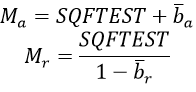

where

   

As with the previous analyses, the quality of each of the three modeled estimates (linear, absolute bias tree, and relative bias tree) was assessed by computing the bias of the modeled estimates compared to the interviewer-measured square footage.

The average modeled square footage from the linear models was 1,927 compared with the measured square footage average of 1,932, which was not a statistically significant difference. Among the 15 subcategories for which comparisons were made, the bias was not statistically significant in approximately half of the categories. Among the eight comparisons in which significant bias was identified, that bias was smaller than the bias of the respondent estimate in nearly all instances. The average bias increased in three instances: apartments in small buildings (increasing from 19 to 132 square feet for the respondent estimated bias and modeled bias, respectively), apartments in large buildings (from 28 to 35 square feet), and housing units with the highest respondent estimates (from 183 to 262 square feet).

In addition to the reduction in average bias, the variability of the bias was also reduced. Overall, the reliability increased from 58.8% for the respondent estimate to 74.7% for the modeled estimate. Each subgroup also saw a reduction in variance and an improvement in the reliability, although the magnitude of the improvement varied from 2.1 percentage points (attached single-family housing units) to 20.5 percentage points (apartments in small buildings). Even given the large reductions, reliability continued to be less than ideal. Moreover, the error was not random. A comparison of the measured square footage estimate with the modeled estimate using linear regression showed larger differences as housing unit size increased.

The regression tree models produced slightly different results than the linear model. Overall, the average bias resulting from the tree of absolute bias was nearly identical to the linear model (average bias of -5 versus 15 square feet for the linear model and absolute bias tree, respectively). Among the subcategory analyses, the absolute bias tree produced biased averages only one-third of the time, slightly better than the linear model. In some cases, the tree of absolute bias performed slightly worse than the linear model, but in other cases it produced slightly more accurate averages.

Among mobile homes, for example, the linear model overestimated average square footage by 10 square feet, whereas the regression tree of absolute bias overestimated the average square footage by 118 square feet. Among apartments in small buildings, this finding was reversed, with the regression tree of absolute bias performing better (average bias of 15 versus -132 square feet, respectively). Although both models resulted in more reliable estimates compared with the respondent report, the linear model improved reliability more in all but one subcategory (housing units with respondent estimates 1,000 square feet or smaller). The linear model may also be considered superior overall because it includes all cases. The regression trees could only be applied to cases for which a respondent estimate was available.

The second regression tree was a model of the relative bias between the respondent report and the measured square footage estimate. Overall, the resulting modeled estimate was 145 square feet lower than the measured square footage estimate. In general, the average absolute bias of the modeled estimate was larger in most cases compared with the absolute bias from either of the other two modeled estimates. However, the relative bias tree produced estimates that had higher reliability than the absolute bias tree nearly two-thirds of the time. When evaluating the relative bias tree on the relative bias of its modeled estimates, it was superior to the linear model and the absolute bias tree in nearly all cases.

In summary, although modeled estimates from the linear models and regression trees were closer to the interviewer measurement than both the respondent and the administrative estimates, they were still significantly different in approximately half of the comparisons. Similarly, they had higher reliability than the respondent and administrative estimates, but the reliability was still low, hovering between 60% and 70%.

Analysis of option to use in-person measured data only

EIA studied the impacts of using only the in-person measured square footage with the in-person sampling weights. Because in-person sampling weights represent the entire population, therefore the in-person square footage measurements can be used to estimate statistics such as average square footage, median square footage, energy consumption per square foot, and total square footage of the U.S. household population.

A major disadvantage to this method is that square footage is an important input to the RECS end-use estimation process; this input would be missing for the self-administered web and paper survey cases. The energy end-use model is used to break down the total, annualized consumption and expenditures for each sampled case into portions used for space heating, air conditioning, water heating, refrigerators, appliances, and other uses.

The equation for each end-use model has total consumption for a fuel (the "known") as the dependent variable, and an appropriate combination of housing unit energy-related characteristics (including square footage), appliance and electronics information, household demographic variables, and weather data as independent variables. The model breaks down (or distributes) the total into end-use components (the "unknown.") Each end-use component is a non-linear expression relating the end-use to its most relevant explanatory variables.

Using the in-person square footage data with its corresponding weights would produce population estimates, but it would not allow end-use estimation, which uses square footage as an input to the model, for web and paper cases.

---

Footnotes

1. Singh, A.C., Grau, E.A., and Folsom, R.E. (2001). “Predictive Mean Neighborhood Imputation with Application to the Person-Pair Data of the National Household Survey on Drug Abuse.” JSM Proceedings, Survey Research Methods Section. Alexandria, VA: American Statistical Association.

2. About 19% of the 2015 in-person surveys did not have sufficient square footage data. This can happen for several reasons: a respondent can refuse to have their home measured, the interviewer may not be able to measure all necessary dimensions (because of factors such as weather or lack of access to certain floors of the home), or EIA can decide that one or more measurements are incorrect during data quality checks.

3. Rubin DB, Schenker N. Multiple Imputation for interval estimation from simple random samples with ignorable nonresponse. Journal of the American Statistical Association. 1986;81 (394):366–374.

4. County real estate records and Realtor.com were considered but not evaluated in this study because they require manual searches, which would be inefficient for capturing data for thousands of records. Trulia.com was also considered. However, Trulia.com was bought by Zillow.com in 2015. The Trulia.com database has been absorbed by Zillow.com, and Trulia.com will soon be dissolved.

Specific questions on this product may be directed to Chip Berry.